S.I.M.P.L.E. Web Interface

Overview

S.I.M.P.L.E. SD combines text-first and diagram-first modeling. Editor checks, diagram highlights, and node tooltips stay synchronized so you can spot issues quickly and fix them from either view.

Single Unified Popup Top-to-Bottom Tour Complete Feature Index Live Search + TOC

Full Interface Tour

This section now includes a real captured interface view, followed by a labeled layout map from top toolbar to output/log surfaces.

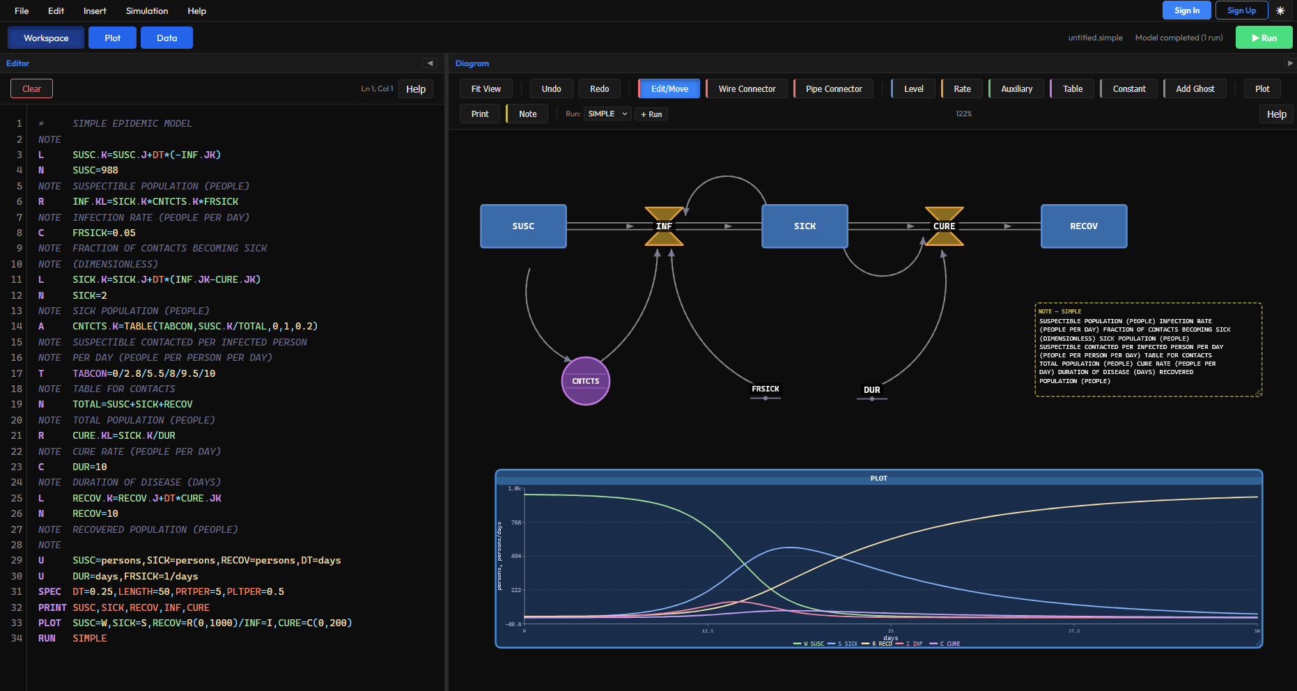
S.I.M.P.L.E. SD interface screenshot showing editor, diagram, and embedded plot node

If any area looks different in your current theme or window size, behavior is still the same: this tour maps the same controls and flow from top bar to output.

Unified Workspace Popup (Editor + Diagram + Plot + Data)

This single help popup combines the main work areas. Use the quick-jump buttons at the top or the table of contents to move between sections without opening separate dialogs.

Editor catches syntax and variable issues with inline code markers.
Diagram mirrors those issues with red node glow and per-node tooltip messages.
Plot displays run-scoped time-series with chip toggles and scales.
Data shows run output rows and CSV export from PRINT variables.

Complete Feature Index

This index lists every major interface area and what it controls.

Area	Includes	Where To Find
Top Menu	File, Edit, Insert, Simulation, Help	App top bar
Workspace Tabs	Workspace, Plot, Data	Main content header
Editor Panel	Code input, code issue underlines, autocomplete, line/column status	Workspace left side
Diagram Panel	Node canvas, wire/pipe drawing, ghosts, notes, plot nodes	Workspace right side
Diagram Toolbar	Move/select/draw modes, node insert tools, run tools, macros	Diagram top row
Context Panel	Name, formula, units, description, apply/delete/hide	When a node is selected
Simulation Settings	DT, LENGTH, PRTPER, PLTPER, RUN, time unit, solver settings	Simulation > Settings
SimRun Replay	Animated diagram replay, dominant loop list, play/pause, slider scrub	Workspace header, next to Run
Plot Tab	Run dropdown, variable chips, line/letter display, hover tooltips	Main Plot tab
Data Tab	PRINT-based output table and CSV export	Main Data tab
Output Log	Parse results, code issue messages, runtime diagnostics	Status/log panel
Cloud/Auth	Sign in/up, cloud save/load model list	Top-right account controls
Help Popup	TOC, search filter, quick jumps, screenshots, references	Help menu and help buttons

Top-to-Bottom Workflow

Define equations in Editor or create nodes in Diagram toolbar.
Use Context Panel Apply to write formulas, units, and descriptions.
Fix any code issue underlines; affected nodes glow red on the diagram.
Use Run for standard output, or SimRun for an animated diagram replay with dominant loop highlighting.
Export CSV or diagram images as needed.

Editor + Code Checks

The editor enforces uppercase style, 72-character line checks, and live code diagnostics. Hover over underlined lines for the exact message.

When a code issue is found, related diagram nodes are highlighted and node tooltip messages are shown in red.

Diagram + Context Panel

The diagram toolbar is organized into labeled sections:

Toolbar Section	Controls
Diagram View	Fit View, Zoom Out (−), Zoom In (+), zoom % display
Edit History	Undo (Ctrl+Z), Redo (Ctrl+Y)
Move Select and Draw	Move/Select (crosshair, default), Wire (dashed info link), Pipe (flow connector), Note (text annotation)
Primary Nodes	Level (rectangle), Rate (valve), Constant (dot + line), Auxiliary (circle)
Special Nodes	Array (stacked rectangles), Table (circle + data lines), Macro (dropdown: + New / list), Ghost (dropdown with variable search), Module scope pill when editing inside a module
Model Output	Plot (embedded chart), Print/Data (data table config)
Run	Run selector dropdown, + Run button, Hidden variables filter

After successful wire or pipe creation, mode returns to Move automatically. Context panel fields sync both directions with editor code, including D descriptions and U units.

Auto-layout: Nodes without saved positions are placed automatically when the diagram opens. The engine groups nodes by subsystem (connected levels and their rates), positions each group, and arranges auxiliaries and constants around them.

Modules: Collapsed module boxes summarize a set of nodes in a standard square box. New modules default to no icon. Click a module to open its settings panel, or double-click it to enter the module's local diagram. Root-view module wires are white dotted proxy links and can be reshaped like other wires.

Draw Modes

Mode	Button	Description
Move / Select	Crosshair (✛)	Default mode. Click to select, drag to reposition. Click empty space to deselect.
Wire	Dashed line	Click source node, then click target to create an information wire (dashed arrow). Adds the source variable to the target's formula dependencies.
Pipe	Solid valve line	Click a level, then a rate (or vice versa) to create a flow pipe (solid connector). Must connect Level ↔ Rate only.
Note	Note icon (📝)	Adds a new note annotation at the next open position on the canvas. Opens the note editor panel.
Lasso	Dashed rectangle	Click and drag to draw a selection rectangle. All nodes inside it are selected together. Selected nodes can be dragged as a group, hidden, or wrapped into a module box.

Lasso Multi-Select

The Lasso tool lets you select multiple nodes at once by drawing a rectangle around them. In the root diagram, selecting two or more model nodes also enables a Create Module action.

Select: Drag a rectangle around nodes to multi-select them (highlighted in blue).
Group drag: After lasso selection, drag any selected node to move the whole group.
Hide: Click the Hide button in the floating action bar to hide all selected nodes at once.
Create Module: In the root view, click Create Module to wrap the selected model nodes in a standard square module box. New modules start with no icon, but you can pick one later in Module Settings.
Open Module: Click a module box to open its settings panel. Double-click the box to enter its local diagram and edit the internal nodes directly.
Module scope: When you are inside a module, the scope pill shows which module you are editing. Exit back to the root view to see collapsed module boxes and proxy links again.
Escape: Press Escape to progressively: cancel active drag → clear selection → exit lasso mode.

Node Types + Shapes

Each variable type has a distinct diagram shape. Below is every node with its visual representation, editor prefix, and usage notes.

Diagram Node	Mode	Shape	Notes
Level	L	Rectangle	Stock/accumulator with N initial value. Integrates flows over time.
Rate	R	Valve/Bowtie	Flow variable connected to levels by pipes. Units derived from connected level.
Auxiliary	A	Circle	Algebraic helper computed each time step. Uses .K timescript.
Table Lookup	A + T	Circle with lines	Auxiliary using TABLE/TABHL/TABXT/TABPL. Data from T line.
Constant	C	Dot + line	Scalar constant, no timescript needed. Can convert to table or array.
Supplementary	S	Dashed triangle	Output-only variable, computed but does not feed back. Uses .K timescript.
Array Level	L + FOR/I	Stacked rectangles	Multi-element stock with index variable and per-element formulas.
Ghost	Reference	Dashed copy	Diagram routing helper. No new equation; reduces long wires.
Plot Node	PLOT	Embedded chart	Run-scoped chart directly on the diagram canvas.
Note Node	O	Note card	Annotation backed by O NTITLE=...,NBODY=... in editor.

Level — Rectangle

Levels (stocks) accumulate flows over time. They require an N initial value and are integrated using the DT time step. The level equation uses .J (previous) and .JK (incoming rates).

L POP.K=POP.J+DT*(BIRTH.JK-DEATH.JK)
N POP=1000

Rate — Valve / Bowtie

Rates define flow between levels. The valve shape has a triangular inlet and a rectangular body. Rates use .KL on the left side and .K on the right side references.

R BIRTH.KL=POP.K*BR

Auxiliary — Circle

Auxiliaries are algebraic computations evaluated each step. They receive information via wires and can feed into rates or other auxiliaries.

A RATIO.K=SICK.K/POP.K

Table Lookup — Circle with Lines

Table nodes are auxiliaries that use a TABLE function. The circle has horizontal data lines to distinguish it from plain auxiliaries. Data values come from a T line.

A EFFECT.K=TABLE(ETAB,INPUT.K,0,100,25)
T ETAB=0/0.2/0.6/0.9/1.0

Constant — Dot + Line

Constants are fixed numeric values that do not change over time. No timescript is needed. They appear as a small dot on a horizontal line.

C BR=0.03

Supplementary — Dashed Triangle

Supplementary variables are output-only computations. They are calculated each step but are not intended to feed back into the model. Useful for reporting derived quantities.

S OUT.K=POP.K*1000

Array Level — Stacked Rectangles

Array levels represent multi-element stocks. They use FOR to declare index variables and I for integer constants. Each element has its own equation expanded at parse time.

FOR AGE=1,3=YOUNG,ADULT,OLD
I NAGES=3
L POP.K(AGE)=POP.J(AGE)+DT*(IN.JK(AGE)-OUT.JK(AGE))

Ghost — Dashed Copy

Ghost nodes are diagram routing helpers. They duplicate the appearance of an existing variable so you can wire it closer to consumers without creating long crossing wires. No new equation is generated.

Plot Node — Embedded Chart

Plot nodes embed a live chart directly on the diagram canvas. They display the time series from the active run's PLOT statement. Click to configure variables, symbols, and scales.

Note Node — Annotation Card

Notes are free-form annotations for documenting parts of the model. They are backed by O statements in the editor with NTITLE and NBODY fields.

O NTITLE=INFECTION RATE,NBODY=PEOPLE PER DAY

Context Panel

The right-side context panel changes by selected element type. Click any node in the diagram to open it.

Panel Mode	Key Fields	Apply Writes
Level Node	Type dropdown, Name, Formula, Units, Description (D), Initial Value (N)	L, N, U, D lines
Rate Node	Type dropdown, Name, Formula, Units (read-only — derived from connected level), Description	R, D lines (unit inferred from level)
Auxiliary Node	Type dropdown, Name, Formula, Units, Description	A, U, D lines
Constant Node	Type dropdown, Name, Formula (numeric value), Units, Description	C, U, D lines
Table Node	Name, TABLE formula, T data (slash-separated), chart preview, Array Const toggle	A + T lines (+ D if set)
Array Node	Size (2–20), Index variable, Element aliases, per-element tabs	FOR, I, expanded L/R per element
Ghost Node	Original variable (read-only), Description, Units, Wire consumer checkboxes	Wire routing only (no equation)
Plot Config	Variables (checkbox list), Symbol letters, Lo/Hi scale values per group	PLOT statement for active run
Print Config	Variables (checkbox list)	PRINT statement for active run
Note	NTITLE and NBODY text fields	O NTITLE=...,NBODY=...

Common controls on all equation panels:

Insert function bar — chip buttons organized by category: Ops (+−*/() DT TIME.K), Math (SQRT, ABS, …), Table (TABLE, TABHL, …), Logic (CLIP, SWITCH, …), Time (STEP, RAMP, PULSE), Delay (DELAY1, SMOOTH, …), plus any user macros.
Connections list — shows inbound wires and pipes with direction, variable name, type, and a remove button.
Hide in diagram — checkbox to visually hide the node while keeping the equation.
Buttons — Apply (writes all changes to editor), Duplicate, Cancel, Delete.

Wires, Pipes + Ghosts

Connections link diagram nodes to represent dependencies. There are two types: information wires and flow pipes.

Connection	Appearance	Valid Between	Effect
Wire	Dashed line with arrow	Any node → Any node	Adds source variable to target's formula dependencies
Pipe	Solid line, optionally with hollow circles	Level ↔ Rate only	Creates flow connection for integration; hollow circles are a diagram display toggle
Module proxy wire	White dotted line at the module box edge	Node ↔ Module or Module ↔ Module (root view)	Represents pending or collapsed module connections and can be curved like other wires

Creating wires: Select Wire mode, click the source node, then click the target. Or Shift+drag from source to target.
Creating pipes: Select Pipe mode, click a level, then a rate (or vice versa).
Module connections: In the root view, you can draw a wire or pipe between a node and a module box, or between two module boxes. That creates a pending module connection shown as a white dotted proxy wire.
Outgoing module wires: Open the source module and use the source node's context panel to assign which internal node owns the outgoing module wire or pipe.
Incoming module wires: Wires going into a module appear inside node panels as Module Imports. Click an import to insert that variable into a formula or initial-value field.
Module-to-module wires: Assign the source side in the source module first. The destination module then exposes that assigned source node as an import in its internal node panels.
Pipe display: Hover and click a pipe to open its settings, then switch between a plain material pipe and a pipe with hollow information markers.
After creation, draw mode automatically returns to Move/Select.
Removing: Select a node, open context panel, and use the remove button next to a connection.
Ghosts are diagram routing helpers. They duplicate a node's appearance at a different position so wires don't cross the whole diagram. No equation is generated.
Ghost nodes can retarget specific consumers — reassigning which consumers read from the ghost's position.

Ghosts are diagram-level routing helpers only. They do not duplicate equations in the model text.

Notes + O Statement

Notes are diagram annotations with title and body, backed by O lines in the editor.

O NTITLE=INFECTION RATE,NBODY=PEOPLE PER DAY / CONTACT DYNAMICS

Rule	Behavior
Both NTITLE and NBODY required	Code checks flag a missing note title or body
Comma separator required	Expected format: O NTITLE=...,NBODY=...
Run scoped	Notes are written into the active run section
Diagram edit sync	Double-click note opens panel and updates O line

S.I.M.P.L.E. SD Extras

D prefix: D VARNAME=DESCRIPTION with X continuation support.
Context field: Variable Description now syncs with D lines.
Tooltip format: description + unit + red error lines.
Error glow: red glow on diagram nodes tied to code issues.
Unit safety: shared U lines are preserved during apply/delete operations.
Insert sync: toolbar and Insert menu include matching elements.

Language Reference

S.I.M.P.L.E. code uses uppercase card-image style statements. Keep statements within 72 characters, start the statement identifier in column 1, and use X for continuation.

*     MODEL TITLE
L     POP.K=POP.J+DT*(BIRTH.JK-DEATH.JK)
N     POP=1000
U     POP=PERSONS,DT=DAYS
D     POP=TOTAL POPULATION

Supported statement families include core equations, metadata cards, run controls, and macro cards:

Family	Statements	Notes
Equations	L, R, A, C, N, T	Core model structure and values
Metadata	U, D, X	Units, descriptions, and continuation lines
Run cards	SPEC, PRINT, PLOT, RUN	Per-run execution and output configuration
Macros	MACRO, INTRN, MEND	Reusable equation templates expanded at parse time

This help follows the S.I.M.P.L.E. code rules used by the editor, including D and O support alongside the core statement families.

Timescripts

Suffix	Meaning	Typical Use
.K	Current time value	Current level/aux states
.J	Previous time value	Level carry-forward term
.JK	Rate from J to K	Flow terms in level integration
.KL	Rate from K to L	Rate equation left-hand side

L POP.K=POP.J+DT*(BIRTH.JK-DEATH.JK)
R BIRTH.KL=POP.K*BR

All Prefixes (L/R/A/C/N/T/S/U/D/O/X/FOR/I)

Prefix	Meaning	Example
L	Level	L POP.K=POP.J+DT*(...)
R	Rate	R BIRTH.KL=POP.K*BR
A	Aux	A RATIO.K=SICK.K/POP.K
C	Const	C BR=0.03
N	Initial	N POP=1000
T	Table data	T TAB=0/1/2/3
S	Supplementary	S OUT.K=POP.K*1000
U	Units	U POP=PERSONS,BR=PERSONS/DAY
D	Description	D POP=TOTAL POPULATION
O	Note payload	O NTITLE=...,NBODY=...
NOTE	Comment line	NOTE TEXT COMMENT
X	Continuation	X CONTINUED TEXT...
FOR	Array index declaration	FOR AGE=1,3=YOUNG,ADULT,OLD
I	Integer/subscript constants	I NAGES=3
SPEC/PRINT/PLOT/RUN	Run control/output cards	SPEC DT=1,... / PRINT ...
MACRO/INTRN/MEND	Macro blocks	MACRO MY(...)

Prefix formatting rules:

Prefix appears in column 1, followed by spaces, then statement text.
Long U and D statements can wrap using one or more X lines.
Variable names are normalized uppercase; unit text is normalized uppercase.

Functions + Operators

All 28 built-in functions. User-defined macros are also callable as functions.

Category	Function	Signature
Math	SQRT	SQRT(x)
	ABS	ABS(x)
	SIN	SIN(x)
	COS	COS(x)
	EXP	EXP(x)
	LOG / LOGN	LOG(x) — natural logarithm
	MAX	MAX(a, b)
	MIN	MIN(a, b)
Table Lookup	TABLE	TABLE(name, input, lo, hi, step)
	TABHL	TABHL(name, input, lo, hi, step) — clamp at bounds
	TABXT	TABXT(name, input, lo, hi, step) — extrapolate beyond bounds
	TABPL	TABPL(name, input, lo, hi, step)
Logic / Conditional	CLIP	CLIP(a, b, x, y) — returns a if x≥y, else b
	SWITCH	SWITCH(a, b, x) — returns a if x=0, else b
	FIFZE	FIFZE(a, b, x) — returns a if x=0, else b
	FIFGE	FIFGE(a, b, x, y) — returns a if x≥y, else b
Delay / Smooth	DELAY1	DELAY1(input, delay) — 1st-order material delay
	DELAY3	DELAY3(input, delay) — 3rd-order material delay
	DELAYP	DELAYP(input, delay, pipeline) — 3rd-order with pipeline output
	DLINF3	DLINF3(input, delay) — 3rd-order information delay
	SMOOTH	SMOOTH(input, delay) — exponential smoothing (1st-order info delay)
Time / Input	STEP	STEP(height, stime) — step input at time stime
	RAMP	RAMP(slope, stime) — ramp starting at stime
	PULSE	PULSE(height, first, interval) — repeating pulse train
Random	NOISE	NOISE() — uniform random [−0.5, 0.5]
Random	NORMRN	NORMRN(mean, stddev) — normal random
Sampling	SAMPLE	SAMPLE(input, interval, start) — sample-and-hold
Array	SUM	SUM(array) — sum all elements
	SUMV	SUMV(array, from, to) — sum range
	PRDV	PRDV(array, from, to) — product of range
	SCLPRD	SCLPRD(a, b, from, to) — scalar product
	SHIFTC / SHIFTL	SHIFTC(a, shift), SHIFTL(a, shift) — circular/linear shift

Operators: + - * / and exponentiation **. Precedence: ** first, then */÷, then +−. Use parentheses to override.

Function Details (from the S.I.M.P.L.E. code manual)

Table Lookups: Express arbitrary relationships between variables using tabulated data points with linear interpolation.

Function	Out of Range Behavior
TABLE	Uses extreme value + warning message
TABHL	Uses extreme value silently (no warning)
TABXT	Extrapolates from last two points (non-horizontal asymptote)
TABPL	Cubic spline interpolation between points. T data needs extra zeros.

A EFFECT.K=TABLE(ETAB,INPUT.K,0,100,25)
T ETAB=0.0/0.3/0.7/0.9/1.0

Delay / Smooth Functions: Model information and material delays in the system.

Function	Type	Description
DELAY1	1st-order material	First-order exponential delay. Output approaches input with single time constant.
DELAY3	3rd-order material	Third-order delay. S-shaped response, more realistic for physical processes.
DELAYP	3rd-order + pipeline	Like DELAY3 but also outputs the total material in the pipeline.
DLINF3	3rd-order information	Information smoothing over three stages.
SMOOTH	1st-order information	Exponential smoothing: SMOOTH.K = SMOOTH.J + DT*(INPUT.JK − SMOOTH.J)/DELAY

Test Input Functions: Generate time-dependent inputs for testing model behavior.

Function	Output Shape	Notes
STEP(H, T)	0 before time T, then H	Sudden one-time change. Both H and T can be variables.
RAMP(S, T)	0 before time T, then accumulating slope S	Linear increase starting at time T.
PULSE(H, F, I)	Pulse of height H, width DT, starting at F, repeating every I	For impulses of area P, use PULSE(P/DT, F, I).
NOISE()	Uniform random [−0.5, +0.5]	Pseudo-random. Same sequence each run unless seed changed.
NORMRN(M, S)	Normal distribution with mean M, stddev S	Max deviation ≈ 2.4 standard deviations.
SAMPLE(X, I, S)	Sample-and-hold: captures X every I time units	Returns initial value S until first sample time.

Trigonometric / Math: Standard mathematical functions. EXP and LOGN can compute arbitrary powers: A^B = EXP(B*LOGN(A)).

Multi-Run Behavior

Models can contain multiple runs (scenarios). The first run is usually the baseline; later runs override only changed statements.

Action	Result
Select run dropdown	Context edits target that run section in the editor
+ Run	Creates a new run section for scenario overrides
Run model	All run sections execute and populate Plot/Data tabs
Settings apply	SPEC settings are synchronized across runs

* BASE RUN
SPEC  DT=1,LENGTH=100,PRTPER=1,PLTPER=1
RUN   BASE

* ALT RUN
R BR.KL=POP.K*0.04
RUN   HIGH BIRTH

Macros

Macros are reusable equation templates. They are defined at the top of the editor and expanded into normal equations when called.

MACRO MYSMOOTH(INPUT,DELAY)
A MYSMOOTH.K=SMOOTH(INPUT.K,DELAY)
MEND

Macro workflow:

Create/edit from the Macro dropdown in the diagram toolbar or directly in code.
Use INTRN for helper names that should be unique for each expansion.
Calls must pass the correct number of arguments.
Macros do not appear as standalone diagram nodes; expanded variables do.

Simulation Settings

Use Settings to configure DT, LENGTH, PRTPER, PLTPER, RUN name, time unit, and integration method (Euler or RK3 with REL_ERR / ABS_ERR).

The Workspace header has two run controls: Run executes the model and updates Plot/Data tabs, while SimRun executes the same model and then opens an animated replay window.

SimRun Replay

SimRun opens a replay window after the model finishes, then animates the diagram slowly so you can see which pipes, rates, and information links are most active over time.

Animated Diagram Replay Play / Pause / Restart Slider Scrubbing Dominant Loop Highlighting

Use the red ▶ SimRun button beside ▶ Run in the Workspace header. SimRun runs the model first, then uses the selected Plot run when available; otherwise it replays the first completed run.

Pipes and wires get wider as relative flow strength increases.
Opacity and glow also respond to the same frame, so weak links fade back while strong links stand out.
The right panel lists the strongest detected feedback loops and highlights the selected loop in orange.
The play button, restart button, and slider let you either watch the replay or scrub through it manually.

SimRun is a visual explanation layer. It does not replace Plot/Data output; it helps reveal when reinforcing or balancing structures dominate during the run.

Plot Tab + Plot Nodes

Run dropdown shows runs with PLOT statements. Diagram plot nodes show run-specific series directly on canvas.

Plot controls include line mode, letter markers, variable chips, and hover readouts. Variables with different magnitudes are normalized by group so traces stay visible.

PLOT Syntax

PLOT  VAR=CHAR(lo,hi)/VAR2=C2(*,*),VAR3=C3(*,*)

=CHAR — assign a single letter symbol that marks the trace (e.g. POP=P).
(lo,hi) — set the Y-axis bounds for this variable. Use * for auto-scale.
/ — separates variables that use different Y-axis scales.
, — groups variables on the same Y-axis scale.

PLOT  POP=P(0,5000)/BIRTH=B(*,*),DEATH=D(*,*)

Above: POP on its own scale 0–5000, BIRTH and DEATH share an auto-scaled axis. Only runs containing a PLOT statement appear in the Plot run dropdown.

Data Tab + CSV Export

Data table includes runs with PRINT statements. Use CSV button to export full output for spreadsheet analysis.

Rows are spaced by PRTPER from SPEC. If PRTPER=0, no print output is produced, so the Data tab stays empty for that run.

PRINT POP,BIRTH,DEATH

Only runs containing a PRINT statement appear in the Data output and CSV export.

Common Errors

Area	Typical Messages	How to Fix
Equations	Undefined variable, missing suffix, malformed assignment	Check spelling, suffixes (.K/.J/.JK/.KL), and equation syntax
Units	Invalid U entries, inconsistent dimensions	Use U NAME=UNIT format and correct each variable entry
Descriptions	D line must be D VARNAME=DESCRIPTION	Keep D format exact; use X lines for long text
Macros	NO MEND CARD, wrong argument count	Close each MACRO with MEND and match call arguments
Run cards	No or incomplete SPEC card	Provide DT, LENGTH, PRTPER, and PLTPER

Code issues are shown in three places at once: editor underline, red node glow, and node tooltip error lines.

Model Examples

Starter examples you can paste and run:

Quick Start

* QUICK START
L POP.K=POP.J+DT*(BIRTH.JK-DEATH.JK)
R BIRTH.KL=POP.K*BR
R DEATH.KL=POP.K*DR
C BR=0.03
C DR=0.02
N POP=1000
U DT=YEAR,POP=PERSONS,BIRTH=PERSONS/YEAR,DEATH=PERSONS/YEAR,BR=1/YEAR,
X DR=1/YEAR
D POP=TOTAL POPULATION
SPEC  DT=1,LENGTH=50,PRTPER=1,PLTPER=1
PRINT POP,BIRTH,DEATH
PLOT  POP=P(0,3000)/BIRTH=B(0,200)/DEATH=D(0,200)
RUN   BASE

Array Cohort Example

This shows a three-element aging chain with one plotted line per array element.

* ARRAY COHORT MODEL
FOR AGE=1,3=YOUNG,ADULT,OLD
L POPULATION.K(AGE)=POPULATION.J(AGE)+DT*(IN.JK(AGE)-OUT.JK(AGE))
R IN.KL(AGE)=SWITCH(BIRTHS,OUT.JK(AGE-1),AGE-1)
R OUT.KL(AGE)=POPULATION.K(AGE)/RESIDENCE(AGE)
A TOTALPOP.K=SUM(POPULATION.K)
C BIRTHS=12
C RESIDENCE(1)=8
C RESIDENCE(2)=22
C RESIDENCE(3)=18
N POPULATION(1)=120
N POPULATION(2)=260
N POPULATION(3)=90
U DT=YEAR,POPULATION=PEOPLE,TOTALPOP=PEOPLE,BIRTHS=PEOPLE/YEAR,
X IN=PEOPLE/YEAR,OUT=PEOPLE/YEAR,RESIDENCE=YEAR
SPEC  DT=1,LENGTH=40,PRTPER=1,PLTPER=1
PRINT TOTALPOP,POPULATION(1),POPULATION(2),POPULATION(3)
PLOT  POPULATION(1)=A,POPULATION(2)=B,POPULATION(3)=C/TOTALPOP=T
RUN   BASE

Macro Smoothing Example

This defines a reusable smoothing macro, then calls it from a normal auxiliary equation.

MACRO MYSMOOTH(INPUT,DELAY)
A MYSMOOTH.K=SMOOTH(INPUT.K,DELAY)
MEND

* MACRO EXAMPLE
A DEMAND.K=STEP(100,5)
A SMOOTHED.K=MYSMOOTH(DEMAND.K,4)
SPEC  DT=0.5,LENGTH=30,PRTPER=1,PLTPER=1
PRINT DEMAND,SMOOTHED
PLOT  DEMAND=D(0,120)/SMOOTHED=S(0,120)
RUN   BASE

Menu Reference

Menu	Items
File	New (Ctrl+N), Open (Ctrl+O), Save (Ctrl+S), Save As (Ctrl+Shift+S), Rename, Export Diagram → SVG / PNG / PDF, Load Example, About
Edit	Undo (Ctrl+Z), Redo (Ctrl+Y)
Insert	Level, Rate, Auxiliary, Table Lookup, Constant, Supplementary, Array, Macro, Ghost, Plot, Print, Note
Simulation	Settings (opens SPEC editor), Run (Ctrl+Enter)
Tools	Dimensional Analysis, Sensitivity Analysis, Feedback Loops, Causes Tree
Help	Manual Help (this panel), Bugs & Feature Requests (GitHub link)

The Workspace header also includes ▶ Run and ▶ SimRun. SimRun is not a menu item; it is a direct replay control that runs the model and opens the animated simulation window.

File Menu Detail

Item	Shortcut	Description
New	Ctrl+N	Clear editor and start a fresh model. Prompts to save unsaved work.
Open	Ctrl+O	Open a model from cloud storage (requires sign-in).
Save	Ctrl+S	Quick save to cloud. If no cloud doc exists yet, opens Save As.
Save As	Ctrl+Shift+S	Save with a new name to cloud storage.
Rename	—	Rename the current cloud model file.
Export → SVG	—	Export the diagram as a scalable SVG file. Best for documentation and editing.
Export → PNG	—	Export the diagram as a 2× resolution PNG image with background fill.
Export → PDF	—	Export the diagram as a single-page PDF with embedded image.
Load Example	—	Load a built-in example model to explore and learn from.
About	—	Version info and application details.

Insert Menu Detail

Every node type from the diagram toolbar is also accessible via the Insert menu. Selecting an item creates the corresponding node on the diagram canvas.

Item	Creates
Level	New L equation and rectangle node
Rate	New R equation and valve node
Auxiliary	New A equation and circle node
Table Lookup	New A+T equation and table circle node
Constant	New C equation and dot+line node
Supplementary	New S equation and dashed triangle node
Array	New array level with FOR/I declarations
Macro	Opens macro dropdown for new/edit
Ghost	Opens ghost dropdown with variable search
Plot	Embedded chart node on diagram
Print	Opens PRINT variable configuration popup
Note	New O statement and annotation card

Tools Overview

The Tools menu provides four analysis tools that help you understand and validate your model's structure and behavior. All tools run against the current editor content.

Dimensional Analysis

Dimensional Analysis checks that your model's unit declarations are self-consistent. It uses U line declarations and propagates units through equations to find mismatches.

Open via Tools → Dimensional Analysis.

How It Works

Parses the current editor source to collect all equations.
Reads declared units from U lines (e.g., U POP=PERSONS,BR=1/YEAR).
Propagates inferred units through equation dependencies.
Checks unit consistency for every equation and flags mismatches.

Output Sections

Section	Shows
Summary	Count of declared units, inferred units, equations checked, pass/warnings
Declared Units	Variables with explicit U line declarations and their types
Inferred Units	Variables whose units were propagated from equation dependencies
No Units	Variables without any unit information (declared or inferred)
Warnings	Unit mismatches found during consistency checking (red border)

Add U declarations to as many variables as possible. The more units you declare, the more comprehensive the analysis.

Sensitivity Analysis

Sensitivity Analysis measures how much a chosen output variable responds to changes in a parameter. It runs three simulations: base, perturbed up, and perturbed down.

Open via Tools → Sensitivity Analysis.

Configuration

Setting	Description
Parameter to perturb	Dropdown of all constants (C) and initial values (N) in the model
Output variable	Dropdown of all levels (L), rates (R), auxiliaries (A), and supplementaries (S)
Perturbation %	The percentage to vary the parameter (1–100%, default 10%)

How It Works

Runs the base simulation with the current parameter value.
Runs a +% simulation with the parameter increased by the perturbation amount.
Runs a −% simulation with the parameter decreased by the perturbation amount.
Shows a trajectory chart comparing all three runs over time.
Calculates elasticity at each time step: (% change in output) / (% change in parameter).

Reading Elasticity

Elasticity	Interpretation
\|E\| < 0.5	Output is insensitive to the parameter — small effect
\|E\| ≈ 1.0	Output changes proportionally — linear relationship
\|E\| > 1.0	Output is highly sensitive — amplified response, leverage point

Sensitivity Analysis excludes SPEC system parameters (DT, LENGTH, PRTPER, PLTPER) from the parameter dropdown.

Feedback Loops

Feedback Loops identifies all circular causal chains in your model. Each loop is classified as Reinforcing (positive feedback) or Balancing (negative feedback) based on link polarities.

Open via Tools → Feedback Loops.

How It Works

Builds an adjacency graph from all equation dependencies (excluding N initial-value equations).
Runs an async depth-first search (chunked for responsiveness) to find cycles up to 12 variables long.
Determines link polarity heuristically: additive references have positive (+) polarity; references in a denominator have negative (−) polarity.
Classifies each loop: an even number of negative links → Reinforcing (R); an odd number → Balancing (B).
Displays up to 2000 unique loops with colored arrows showing each link's polarity.

Understanding Loop Polarity

Symbol	Meaning
→(+)	Positive link: as the source increases, the target increases (or decreases together)
→(−)	Negative link: as the source increases, the target decreases (appears in denominator or subtracted)
R	Reinforcing: even number of negative links → self-amplifying feedback
B	Balancing: odd number of negative links → self-correcting feedback

Use the filter dropdown to show only loops containing a specific variable.
Maximum loop length is 12 variables. Maximum displayed loops is 2000.
Progress is shown during search: "X found so far (Y% scanned)".

Causes Tree

The Causes Tree traces all upstream dependencies for a chosen variable, displayed as an SVG tree diagram using the same node shapes as the main diagram.

Open via Tools → Causes Tree.

Configuration

Setting	Description
Select a variable	Dropdown of all model variables (excluding N initial values)
Depth	How many levels deep to trace (2–6, default 4)

Tree Features

Node shapes match diagram: Levels = rectangles, Rates = valves, Auxiliaries = circles, Constants = dot+line.
Circular references: Marked with a dashed border and ↻ symbol to prevent infinite recursion.
Zoom controls: Use +, −, and ⊙ (reset) buttons to zoom the tree view.
Theme-aware: Tree adjusts to light or dark mode automatically.

Export Diagram

Export the current diagram to an image file via File → Export Diagram.

Format	Best For	Details
SVG	Documentation, editing	Scalable vector format. Inline styles included. Can be opened in design tools for further editing.
PNG	Presentations, sharing	Rendered at 2× resolution for high-DPI displays. Background color matches your theme.
PDF	Printing, reports	Single-page PDF with embedded image. Uses the diagram's bounding box as page size.

All exports are auto-cropped to the diagram content with padding. Hidden nodes are excluded. The file downloads automatically to your Downloads folder.

Cloud Save / Load

S.I.M.P.L.E. SD supports cloud storage for your models. Sign in with email/password or Google to save and access models from any device.

Authentication

Sign In / Sign Up: Use the top-right button or the welcome screen. Supports email+password and Google OAuth.
Once signed in, the button changes to show your account with Save and My Models options.

Cloud Operations

Action	How	Description
Save	Ctrl+S or File → Save	Quick save to cloud. If no cloud document exists yet, opens Save As.
Save As	Ctrl+Shift+S or File → Save As	Save with a new name. Enter a model name in the dialog and confirm.
Open	Ctrl+O or File → Open	Opens My Models list showing all saved models, sorted by last modified date.
Rename	File → Rename	Rename the current cloud model file (copies to new name, deletes old).
Delete	My Models list	Each model in the list has a delete button for removing unwanted models.

Cloud saves include the diagram layout (node positions). When you open a cloud model, nodes appear exactly where you left them.

Autocomplete

The editor provides live autocomplete suggestions as you type. Suggestions include variable names, system constants, functions, keywords, and timescripts.

Suggestion Categories

Icon	Category	Examples
V	User variable	POP, BIRTH, RATIO — names from your model equations
S	System constant	DT, TIME, LENGTH, PRTPER, PLTPER
F	Function	SQRT, TABLE, CLIP, DELAY1, STEP, PULSE, etc. (opens parenthesis on accept)
K	Keyword	L, R, A, C, N, S, T, U, SPEC, PRINT, PLOT, RUN, NOTE, MACRO
T	Timescript	.K, .J, .KL, .JK — appears after typing a dot (.)

Usage

Start typing to see suggestions — minimum 1 character triggers the popup.
Use ↑/↓ arrow keys to navigate the list.
Press Tab or Enter to accept the highlighted suggestion.
Press Escape to dismiss the popup.
After a dot (.), timescript suggestions appear ranked by variable type (e.g., levels show .K/.J first, rates show .KL first).
Accepting a function inserts the name followed by an opening parenthesis.

Shortcuts + Tips

Shortcut	Action
Ctrl+Enter	Run model
Space (inside SimRun)	Play / pause replay
Ctrl+Z	Undo
Ctrl+Y / Ctrl+Shift+Z	Redo
Ctrl+N	New model
Ctrl+O	Open model (cloud load)
Ctrl+S	Save
Ctrl+Shift+S	Save As
Tab	Insert 6 spaces / accept autocomplete
Enter	Accept autocomplete selection
Escape	Close dialog or SimRun / cancel draw mode / deselect node / dismiss autocomplete
Delete	Delete selected diagram element
Shift+Drag	Quick wire placement between nodes
↑ / ↓	Navigate autocomplete suggestions

Editor Tips

Use ghost variables to reduce long wires across the diagram.
Use Fit View when the diagram pans far from center.
Autocomplete suggestions appear as you type variable and function names. Timescript suggestions appear after a dot.
The column-72 ruler (dashed red line) marks the S.I.M.P.L.E. code line length limit. Use X continuation lines for longer statements.
Code issues appear in three synchronized places: editor underline, diagram node glow, and node tooltip.
The editor enforces uppercase style for all code. Variable names and units are normalized automatically.

Diagram Tips

Double-click a node to open its context panel for editing.
Right-click a node to access quick actions.
Use the Lasso tool to select and move or hide multiple nodes at once.
Zoom with the +/− buttons or fit the entire model with Fit View.
Wires show information flow (dashed lines). Pipes show material flow (solid lines).
Hidden nodes can be restored from the "Hidden" dropdown in the Run toolbar section.

Model Tips

A model needs at minimum: one equation, a SPEC card, and a RUN card.
Add U declarations for unit checking. Use D declarations for documentation.
Use Sensitivity Analysis to find which parameters have the most impact.
Use Feedback Loops to understand the causal structure of your model.
Use Dimensional Analysis to catch unit errors early.
Save frequently to the cloud. Your diagram layout is preserved with the model.

Unified S.I.M.P.L.E. code documentation

Dominant Loops

S.I.M.P.L.E. Code Help

Overview

Full Interface Tour

Unified Workspace Popup (Editor + Diagram + Plot + Data)

Complete Feature Index

Top-to-Bottom Workflow

Editor + Code Checks

Diagram + Context Panel

Draw Modes

Lasso Multi-Select

Node Types + Shapes

Level — Rectangle

Rate — Valve / Bowtie

Auxiliary — Circle

Table Lookup — Circle with Lines

Constant — Dot + Line

Supplementary — Dashed Triangle

Array Level — Stacked Rectangles

Ghost — Dashed Copy

Plot Node — Embedded Chart

Note Node — Annotation Card

Context Panel

Wires, Pipes + Ghosts

Notes + O Statement

S.I.M.P.L.E. SD Extras

Language Reference

Timescripts

All Prefixes (L/R/A/C/N/T/S/U/D/O/X/FOR/I)

Functions + Operators

Function Details (from the S.I.M.P.L.E. code manual)

Multi-Run Behavior

Macros

Simulation Settings

SimRun Replay

Plot Tab + Plot Nodes

PLOT Syntax

Data Tab + CSV Export

Common Errors

Model Examples

Quick Start

Array Cohort Example

Macro Smoothing Example

Menu Reference

File Menu Detail

Insert Menu Detail

Tools Overview

Dimensional Analysis

How It Works

Output Sections

Sensitivity Analysis

Configuration

How It Works

Reading Elasticity

Feedback Loops

How It Works

Understanding Loop Polarity

Causes Tree

Configuration

Tree Features

Export Diagram

Cloud Save / Load

Authentication

Cloud Operations

Autocomplete

Suggestion Categories

Usage

Shortcuts + Tips

Editor Tips

Diagram Tips

Model Tips

🚀 Welcome to S.I.M.P.L.E. SD

📚 Example Models